Enhancing the Performance of Solar Radiation Decomposition Models Using Deep Learning

Rial Arifin Rajagukguk; Hyunjin Lee

doi:10.7836/kses.2023.43.3.073

Preview

Research Article

Journal of the Korean Solar Energy Society. 30 June 2023. 73-86
https://doi.org/10.7836/kses.2023.43.3.073

Enhancing the Performance of Solar Radiation Decomposition Models Using Deep Learning

Rial Arifin Rajagukguk¹

Hyunjin Lee²^*

¹Graduate Student, School of Mechanical Engineering, Kookmin University

²Professor, School of Mechanical Engineering, Kookmin University

^{*Corresponding Author}

ABSTRACT

Decomposed solar radiation models are commonly used to separate direct and diffuse irradiance from global irradiance. However, most of these models are designed to process hourly data, which may not be sufficient to capture the rapid changes in solar irradiance that occur within a shorter timescale. To address this issue, we examined the performance of existing decomposition models at different temporal resolutions ranging from 1 min to 1 h. We found that the errors in the decomposition models increased as the temporal resolution decreased. Specifically, as the timescale was reduced from hourly to every minute, the relative root-mean-square error (rRMSE) increased by more than 5%. These findings highlight the need to develop accurate models that can process sub-hourly data. Accordingly, we propose the use of deep learning models to estimate the direct irradiance using sub-hourly data. The proposed models significantly reduced the rRMSE by more than 7% compared to the existing models on a 1-min time scale. The results indicate that deep-learning models can provide accurate estimates of direct irradiance, even at sub-hourly temporal resolutions.

Keywords

Direct normal irradiance

Decomposition model

Deep learning

Temporal resolutions

키워드

법선면 직달 일사량

직산분리 모델

딥러닝

시간 분해능

MAIN

1. Introduction
2. Data description
3. Decomposition model
3.1 Erbs
3.2 Reindl
3.3 Maxwell
3.4 Perez
4. Deep learning model
4.1 LSTM
4.2 GRU
5. Results and Discussion
6. Conclusions

Abbreviations

DNI : Direct normal irradiance (W/m²)

DHI : Diffuse horizontal irradiance (W/m²)

GHI : Global horizontal irradiance (W/m²)

GRU : Gated recurrent unit

LSTM : Long short-term memory

QC : Quality control

rMBE : Relative mean bias error (%)

rRMSE : Relative mean square error (%)

Nomenclature

$E_{a}$ : Extraterrestrial irradiance (W/m²)

$k_{t}$ : Clearness index

$k_{d}$ : Diffuse fraction

$k_{n}$ : Direct beam transmission

$k_{t c}$ : Clear sky index

$m_{a}$ : Air mass

1. Introduction

Solar irradiance components such as global horizontal irradiance (GHI), direct normal irradiance (DNI), and diffuse horizontal irradiance (DHI) are important for solar energy applications. The GHI is important as a resource of solar energy information to provide greater photovoltaic (PV) power production under all sky conditions. DNI is an important component of global irradiance, particularly under cloudless situations, and it represents a solar resource that may be exploited by many types of concentrating solar technology (CST)¹⁾. DHI is also important because it is required for energy and building applications²⁾. However, most solar irradiance measurements solely focus on GHI because the devices to measure DHI and DNI are costly. Furthermore, the devices such as a pyrheliometer to measure DNI require periodic maintenance and calibration because they are mounted on a sun tracker that moves according to the sun's position.

Over the past half-century, decomposition solar radiation models have been developed to estimate DNI and DHI in order to obtain a more accurate estimate of solar irradiance components. Most of the decomposition models use correlations between clearness index and diffuse fraction. The following formula is used to calculate the clearness index and diffuse fraction.

(1)

k_{t} = \frac{GHI}{E_{a} \cos θ_{z}}

(2)

k_{d} = \frac{DHI}{GHI}

where $k_{t}$ denotes the clearness index, $k_{d}$ indicates the diffuse fraction, $E_{a}$ denotes the extraterrestrial irradiance, and $θ_{z}$ represents the solar zenith angle. However, a major limitation of most of these models is that they have primarily been developed for hourly global solar radiation data. This presents a challenge for solar energy applications, as sub-hourly data are required to accurately estimate the rapid changes in solar irradiance that occur over short time intervals. Despite the importance of sub-hourly data for solar energy applications, there has been relatively little research on the development of decomposition models that can handle this level of temporal resolution. This has led to a reliance on hourly data, which may not capture the true variability of solar irradiance over shorter time intervals. The lack of accurate sub-hourly data has also led to limitations in the design and optimization of solar energy systems. Without accurate information on the rapid changes in solar irradiance, it is difficult to optimize the performance of solar energy systems and ensure maximum power generation.

Therefore, in this study, we evaluated the accuracy of well-known decomposition models using sub-hour solar irradiance data. The decomposition models are evaluated at several temporal resolutions (1 hr, 30 min, 15 min, 5 min, 1 min) to estimate DNI using solar irradiance data in Korea. In addition, the estimated DNI using the decomposition model is compared with deep learning models to determine which model is best suited for sub-hourly data resolution.

2. Data description

The instruments to measure GHI, DHI, and DNI were set up on the rooftop at Kookmin University in Seoul, South Korea (latitude: 37.61200° N, longitude: 126.99770° E). Solar irradiance data in 2021 are used in this study. Furthermore, to acquire the best and most accurate solar irradiance ground measurement data, a set of quality control (QC) and explicit standards are required. Data QC is the use of techniques or processes to determine if data meets overall quality goals and particular quality requirements. A set of QC procedures that adhere to the baseline surface radiation network (BSRN) recommended³⁾ QC tests are provided below.

1. $θ_{z}$ < 85°

2. 0 < GHI < 1.50 $E_{a}$ cos^1.2 $θ_{z}$ + 100 Wm^-2

3. 0 < DHI < 0.95 $θ_{z}$ cos^1.2 $θ_{z}$ + 50 Wm^-2

4. 0 < DNI < $E_{a}$ Wm^-2

5. Abs[(DNIcos $θ_{z}$ + DHI ‒ GHI) / GHI] < 0.08; for $θ_{z}$ < 75° and GHI > 50 Wm^-2

6. Abs[(DNIcos $θ_{z}$ + DHI ‒ GHI) / GHI] < 0.15; for $θ_{z}$ ≥ 75° and GHI > 50 Wm^-2

7. DHI / GHI < 1.05; for $θ_{z}$ < 75° and GHI > 50 Wm^-2

8. DHI / GHI < 1.10; for $θ_{z}$ ≥ 75° and GHI > 50 Wm^-2

Condition (1) when ( $θ_{z}$ < 85°) is included to eliminate the low irradiance. This is due to the fact that the errors for solar radiation models are large at low solar elevations⁴⁾. As a result, to achieve a good quality of data the data points that do not satisfy the QC procedure will be eliminated.

3. Decomposition model

3.1 Erbs

Erbs et al.⁵⁾ introduced a correlation method that uses solar irradiance data from five different locations in the United States. They calculated hourly, daily, and monthly averages of this data to create a fourth-order polynomial equation. The equations of the Erbs model are expressed as:

(3)

k_{d} = \{\begin{cases} 0.9511 - 0.1604 k_{t} + 4.388 {k_{t}}^{2} - 16.638 {k_{t}}^{3} + 12.336 {k_{t}}^{4} & 0.22 < k_{t} < 0.80 \\ 1.0 - 0.09 k_{t} & k_{t} \leq 0.22 \\ 0.165 & k_{t} > 0.80 \end{cases}

3.2 Reindl

The Reindl⁶⁾ model was created using data from five European and North American regions, and the solar zenith angle was introduced as a second input parameter to estimate diffuse fraction in addition to the clearness index.

(4)

k_{d} = \{\begin{cases} 1.02 - 0.254 k_{t} + 0.0123 \cos θ_{z} & k_{t} \leq 0.3 \\ 1.4 - 1.749 k_{t} + 0.177 \cos θ_{z} & 0.3 < k_{t} < 0.78 \\ 0.486 k_{t} - 0.182 \cos θ_{z} & k_{t} \geq 0.78 \end{cases}

3.3 Maxwell

The Maxwell model⁷⁾, commonly known as the direct insolation simulation code (DISC) model, uses an exponential connection between direct beam transmittance and air mass and contains correlation functions with a parameter of clearness index. The primary variable influencing the connection between and is air mass, which may be computed using clear-sky direct beam transmittance and deviations from clear transmittance values.

(5)

k_{n} = k_{n c} - ∆ k_{n}

(6)

k_{n c} = 0.866 - 0.122 m_{a} + 0.0121 m_{a}^{2} - 0.000653 m_{a}^{3} + 0.000014 m_{a}^{4}

(7)

∆ k_{n} = A + B \exp (C m_{a})

where $k_{n}$ is direct beam transmittance, and $m_{a}$ is air mass, $k_{n c}$ is clear-sky direct beam transmittance, $∆ k_{n}$ is deviations from clear transmittance values, and $A$ , $B$ , $C$ are polynomial functions dependent on the clearness index.

3.4 Perez

To enhance the Maxwell model, the Perez model⁸⁾ was created. The outcome of this model was given a correction coefficient function of normalized clearness index, solar zenith angle, and precipitable water to the result of Maxwell model.

(8)

I_{b n} = I_{b n} (DISC) X (k'_{t}, θ_{z}, δ k'_{t}, W)

(9)

k'_{t} = \frac{k_{t}}{1.031 \exp (\frac{- 1.14}{0.9 + 9.4 m_{a}^{- 1}}) + 0.1}

(10)

δ k'_{t} = \frac{| k'_{t_{i}} - k'_{t_{i + 1}} | + | k'_{t_{i}} - k'_{t_{i - 1}} |}{2}

Here, $k'_{t}$ is the normalized clearness index, $I_{b n}$ is direct normal irradiance, and $W$ is precipitable water.

4. Deep learning model

4.1 LSTM

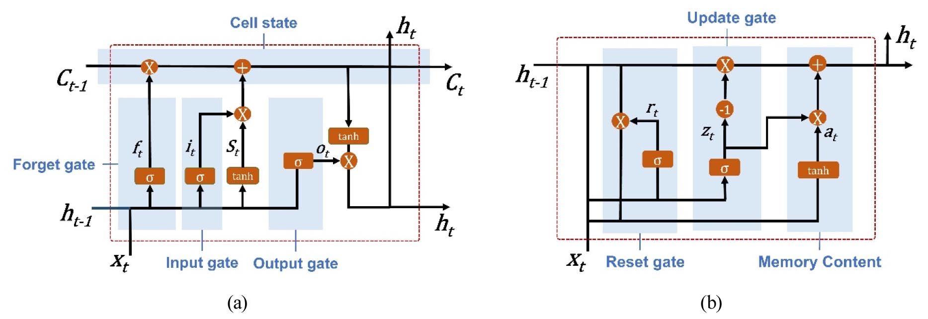
Long-short term memory (LSTM) was first introduced by Hochreiter et al.⁹⁾ as a temporal recurrent neural network (RNN) for learning long-term information dependence. When training a simple RNN, issues with vanishing and exploding gradients arise when the data sequence is too long to carry the information. Thus, the LSTM model was established to address these problems. The operation inside the cells of LSTM consists of three gates: input, output, and forget as shown in Fig. 1(a). It aids in either remembering or forgetting information via the forget gate, solving the vanishing and exploding gradient problems associated with long-distance information transmission.

(11)

f_{t} = σ (ω_{f} x_{t} + u_{f} L_{t - 1} + b_{f})

(12)

i_{t} = σ (ω_{i} x_{t} + u_{i} L_{t - 1} + b_{i})

(13)

S_{t} = \tanh (ω_{c} x_{t} + u_{c} L_{t - 1} + b_{c})

(14)

O_{t} = σ (ω_{o} x_{t} + u_{o} L_{t - 1} + u_{o} L_{t - 1} + b_{o})

(15)

L_{t} = O_{t} + \tanh (S_{t})

(16)

C_{t} = i_{t} S_{t} + f_{t} S_{t - 1}

where $f_{t}$ is the forget gate, $i_{t}$ is the input gate, $S_{t}$ is the value of candidate state memory, $C_{t}$ is the state of the memory cell, $O_{t}$ is the output gate, $σ$ and $\tanh$ are the activation functions, and $L_{t}$ is the final memory at the current time step.

4.2 GRU

Cho et al.¹⁰⁾ proposed gated recurrent unit (GRU) as a more straightforward RNN architecture than LSTM. To remember important details and capture long-term dependencies, GRU is comparable to LSTM. GRU's strength lies in the fact that it is less complicated and takes less time to compute than LSTM, because it has fewer parameters. Therefore, GRU can be trained much more quickly than LSTM. GRU has two gates: update gate and reset gate. The amount of data that must be lost from the past is set by the reset gate, while the type of data that should be stored for the future is set by the update gate.

Fig. 1(b) depicts the architecture of the GRU’s cell, and the following equation describes the connection between GRU's inputs and outputs.

(17)

r_{t} = σ (ω_{r} x_{t} + u_{r} g_{t - 1} + b_{r})

(18)

z_{t} = σ (ω_{z} x_{z} + u_{z} g_{t - 1} + b_{z})

(19)

a_{t} = \tanh (ω_{h} x_{t} + u_{h} r_{t} g_{t - 1} + b_{h})

(20)

g_{t} = (1 - z_{t}) g_{t - 1} + z_{t} a_{t}

where $r_{t}$ is the reset gate, $Z_{t}$ is the update gate, $A_{t}$ is the memory content, $σ$ and $\tanh$ are the activation functions, and $g_{t}$ is the final memory at the current time step.

https://cdn.apub.kr/journalsite/sites/kses/2023-043-03/N0600430307/images/kses_2023_433_73_F1.jpg

Fig. 1

The architecture of deep learning models: (a) LSTM and (b) GRU

5. Results and Discussion

The evaluation metrics used to evaluate the accuracy of the decomposition and deep learning models are relative root mean square error (rRMSE) and relative mean bias error (rMBE). Evaluation metrics that measure relative performance are preferred because they show percentage error and are thus more useful when data vary with time scale.

(21)

rMBE = \frac{\frac{1}{n} \sum_{i = 1}^{n} (y_{e} - y_{m})}{{\bar{y}}_{m}}

(22)

rRMSE = \frac{\sqrt{\frac{1}{n} \sum_{i = 1}^{n} (y_{e} - y_{m})^{2}}}{{\bar{y}}_{m}},

(23)

R^{2} = 1 - \frac{\sum_{i = 1}^{n} (y_{e} - y_{m})^{2}}{\sum_{i = 1}^{n} (y_{e} - {\bar{y}}_{m})^{2}}

where $y_{m}$ , $y_{e}$ , $y_{m}$ , $n$ represents the actual output, estimated output, mean value of, mean value of actual output, and the number of samples respectively.

Fig. 2 shows the results of decomposition solar radiation models to estimate DNI at various temporal resolutions. All decomposition models tend to have greater error as the time scale decreases. Using every minute and hourly solar irradiance data, the rRMSE difference error for all models is greater than 4%. Table 1 provides a comprehensive summary of the results of decomposition models for different sky conditions. The sky conditions are categorized based on the clearness index value¹¹⁾. The sky conditions are divided into the overcast sky ( $k_{t} \leq 0.35$ ), partly cloudy ( $0.35 < k_{t} < 0.65$ ), and overcast sky ( $k_{t} \geq 0.65$ ). It indicates that the rRMSE values are the highest when using every minute data, while the hourly data produces the most accurate results in all-sky conditions. For this reason, deep learning models are used to estimate DNI from minute-level irradiance data in order to improve the performance of decomposition models.

https://cdn.apub.kr/journalsite/sites/kses/2023-043-03/N0600430307/images/kses_2023_433_73_F2.jpg

Fig. 2

rRMSE of decomposition models to estimate DNI at different temporal resolutions

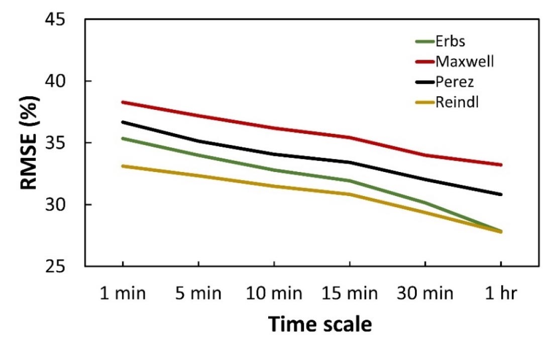
Table 1

rRMSE of decomposition models at different temporal resolutions for various sky conditions

	rRMSE (%)
	Erbs	Maxwell	Perez	Reindl
Overcast sky ( $k_{t} \leq 0.35$ )
1 min	456.5	462.1	442.3	448.2
5 min	403.7	401.8	369.7	397.0
10 min	370.0	370.4	333.6	366.2
15 min	345.5	341.7	311.0	339.1
30 min	276.9	309.2	263.9	294.4
1 hr	231.7	275.1	267.1	259.1
Partly cloudy ( $0.35 < k_{t} < 0.65$ )
1 min	41.4	44.9	41.9	38.7
5 min	40.4	43.8	40.8	37.7
10 min	39.3	42.6	40.2	36.6
15 min	38.9	41.8	39.9	36.0
30 min	37.0	40.5	39.0	34.2
1 hr	33.4	39.7	37.1	31.4
Overcast sky ( $k_{t} \geq 0.65$ )
1 min	21.4	23.2	22.5	20.0
5 min	20.2	22.3	21.3	19.4
10 min	19.3	21.7	20.4	18.9
15 min	18.4	21.0	19.7	18.3
30 min	17.3	20.0	18.5	17.5
1 hr	16.0	19.2	17.7	16.7

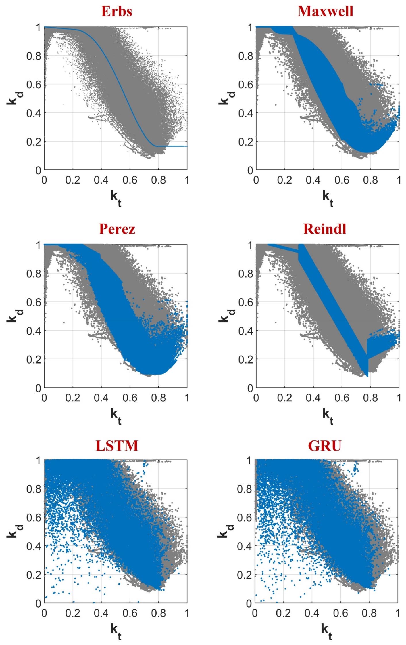
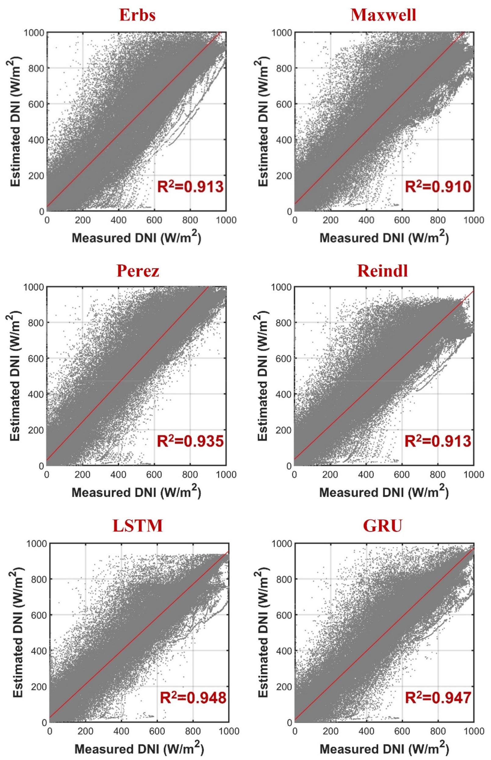
In decomposition and deep learning models, the correlation between the clearness index and the diffuse fraction is crucial for determining whether the model functions well. The difference between the decomposition and deep learning models can be seen in Fig. 3. It shows that decomposition models cannot cover the gray distribution, which represents the actual measured data. The deep learning models, on the other hand, demonstrated better results and showed high coverage. The scatter plot of the estimated and measured DNI of the decomposition and deep learning models is depicted in Fig. 4. Compared to decomposition models, the accuracy of deep learning models was observably enhanced. It demonstrates that the GRU and LSTM models outperform all decomposition models, with the coefficient of determination (R²) values of 0.947 and 0.948, respectively.

https://cdn.apub.kr/journalsite/sites/kses/2023-043-03/N0600430307/images/kses_2023_433_73_F3.jpg

Fig. 3

Scatterplots of the clearness index ( $k_{t}$ ) and diffuse fraction ( $k_{d}$ ) of the decomposition and deep learning models at 1-minute data resolution. The gray and blue points represent the measured and model, respectively

https://cdn.apub.kr/journalsite/sites/kses/2023-043-03/N0600430307/images/kses_2023_433_73_F4.jpg

Fig. 4

Scatterplots of decomposition and deep learning models to estimate DNI at 1-minute data resolution

For greater comprehension, the comprehensive outcomes of each model are presented in Table 2, offering a detailed review. Additionally, Fig. 5 illustrates the variations in patterns observed in each model as the time scale is changed. In terms of rRMSE, the deep learning models outperformed all decomposition models, where the error is approximately 25% in every minute data resolution. The deep learning models also have the smallest value of rMBE, with values of -0.7% and -1.9% for GRU and LSTM, respectively. However, as the time scale increases, the accuracy of deep learning models decreases. For example, the rRMSE for LSTM rises to 27.0% when the data resolution is every 15 minutes and 27.5% using hourly data resolution. In contrast to decomposition models, the accuracy of all models improves as the time scale increases. Compared to minute data resolution, the rRMSE of decomposition models decreases by approximately 3% when using 15-minute data resolution and by approximately 5% when using hourly data resolution.

Table 2

rRMSE and rMBE of decomposition and deep learning models at different temporal resolutions

Model	1 min		5 min		10 min		15 min		30 min		1 hr
Model	rRMSE (%)	rMBE (%)	rRMSE (%)	rMBE (%)	rRMSE (%)	rMBE (%)	rRMSE (%)	rMBE (%)	rRMSE (%)	rMBE (%)	rRMSE (%)	rMBE (%)
Erbs	35.4	-10.7	34.0	7.9	32.8	7.1	31.9	6.5	30.2	5.6	27.8	4.6
Maxwell	38.3	15.2	37.2	14.0	36.2	13.2	35.4	12.6	34.0	11.7	33.2	11.3
Perez	36.7	17.6	35.1	16.6	34.1	15.6	33.4	14.5	32.0	13.6	30.8	12.4
Reindl	33.1	5.9	32.3	5.2	31.5	4.5	30.8	4.0	29.4	3.4	27.8	2.8
LSTM	25.3	-1.9	25.6	1.4	26.5	3.1	27.0	-2.2	27.1	-6.2	27.5	-7.0
GRU	25.3	-0.7	25.5	1.0	26.2	-1.5	27.4	-1.7	27.7	3.3	28.6	-5.0

https://cdn.apub.kr/journalsite/sites/kses/2023-043-03/N0600430307/images/kses_2023_433_73_F5.jpg

Fig. 5

rRMSE of decomposition and deep learning models to estimate DNI at different temporal resolutions

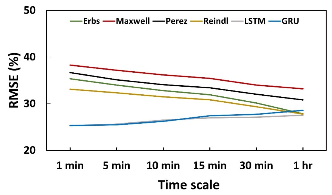
6. Conclusions

To assess the accuracy of the decomposition solar radiation models in estimating DNI at various temporal resolutions, four such models were employed. The findings indicated an increase in error as the temporal scale was reduced to sub-hour intervals, with the rRMSE increasing by more than 4% when the temporal scale was reduced from hourly to minutely. The decomposition models exhibited rRMSE results exceeding 33% at every minute time scale. To improve the accuracy of DNI estimation, deep learning models such as GRU and LSTM were utilized as a solution. The results demonstrate that the deep learning models outperform the decomposition models across all temporal resolutions, with the rRMSE value being less than 26% and 29% for 1-minute and 1-hour temporal resolutions, respectively. However, due to a reduction in training data, deep learning models' accuracy decreased as the temporal scale increased. The results indicate that deep learning models are more suitable for estimating DNI at sub-hourly intervals. Moreover, these outcomes offer valuable insights into the effectiveness of decomposition and deep learning models in estimating solar radiation. This information can facilitate the creation of more precise models for assessing solar resources, which can have implications for the development and optimization of solar energy systems.

Acknowledgements

This research was supported by the Ministry of Trade, Industry & Energy (MOTIE), Korea Evaluation Institute of Industrial Technology (KEIT) through the Vehicle Industry Technology Development Program (20018646).

References

Law, E. W., Prasad, A. A., Kay, M., and Taylor, R. A., Direct Normal Irradiance Forecasting and Its Application to Concentrated Solar Thermal Output Forecasting - A Review, Sol. Energy, Vol. 108, pp. 287-307, 2014, https://doi.org/10.1016/j.solener.2014.07.008. 10.1016/j.solener.2014.07.008

de Simón-Martín, M., Alonso-Tristán, C., and Díez-Mediavilla, M., Diffuse Solar Irradiance Estimation on Building’s Façades: Review, Classification and Benchmarking of 30 Models under All Sky Conditions, Renew. Sustain. Energy Rev., Vol. 77, pp. 783-802, 2017, https://doi.org/10.1016/j.rser.2017.04.034. 10.1016/j.rser.2017.04.034

Frostinger, A., Wilbert, S., Jensen, A. R., Kraas, B., Peruchena, C. F., Gueymard, C. A., Ronzion, D., Yang, D., Collino, E., Martinez, J. P., Ruiz-Arias, J. A., Hanrieder, N., Blanc, P., and Saint-Drenan, Y., Expert Quality Control of Solar Radiation Ground Data Sets, Proceedings of the International Solar Energy Society (ISES) Solar World Congress, pp. 1037-1048, October 2021, online, France, https://doi.org/10.18086/swc.2021.38.02. 10.18086/swc.2021.38.02

Yang, D., Estimating 1-min Beam and Diffuse Irradiance from the Global Irradiance: A Review and an Extensive Worldwide Comparison of Latest Separation Models at 126 Stations, Renew. Sustain. Energy Rev., Vol. 159, 112195, 2022, https://doi.org/10.1016/j.rser.2022.112195. 10.1016/j.rser.2022.112195

Erbs, D. G., Klein, S. A., and Duffie, J. A., Estimation of the Diffuse Radiation Fraction for Hourly, Daily and Monthly-average Global Radiation, Sol. Energy, Vol. 28, No. 4, pp. 293-302, 1982, https://doi.org/10.1016/0038-092X(82)90302-4. 10.1016/0038-092X(82)90302-4

Reindl, D. T., Beckman, W. A., and Duffie, J. A., Diffuse Fraction Correlations, Sol. Energy, Vol. 45, pp. 1-7, 1990, https://doi.org/10.1016/0038-092X(90)90060-P. 10.1016/0038-092X(90)90060-P

Maxwell, E. L., A Quasi-physical Model for Converting Hourly Global Horizontal to Direct Normal Insolation, Sol. Energy Res. Institute, 1987.

Perez, R. R., Ineichen, P., Maxwell, E. L., Seals, R. D., and Zelenka, A., Dynamic Global-to-direct Irradiance Conversion Models, ASHRAE Trans., Vol. 98, pp. 354-369, 1992.

Hochreiter, S. and Schmidhuber, J., Long Short-Term Memory, Neural Comput., Vol. 9, No. 8, pp. 1735-1780, 1997, https://doi.org/10.1162/neco.1997.9.8.1735. 10.1162/neco.1997.9.8.1735

Cho, K., van Merriënboer, B., Gulcehre, C., Bahdanau, D., Bougares, F., Schwenk, H., and Bengio, Y., Learning Phrase Representations using RNN Encoder-decoder for Statistical Machine Translation, Proceedings of the 2014 Conference on Empirical Methods in Natural Language Process (EMNLP), pp. 1724-1734, October 2014, Doha, Qatar, https://doi.org/10.3115/v1/d14-1179. 10.3115/v1/d14-1179

Rajagukguk, R. A., Choi, W. K., and Lee, H., Sun-blocking Index from Sky Image to Estimate Solar Irradiance, Build. Environ., Vol. 223, 109481, 2022, https://doi.org/10.1016/j.buildenv.2022.109481. 10.1016/j.buildenv.2022.109481

Journal of the Korean Solar Energy Society ISSN:1598-6411(Print) 2508-3562(Online) 한국태양에너지학회 논문집

Preview

Enhancing the Performance of Solar Radiation Decomposition Models Using Deep Learning

ABSTRACT

MAIN

(1)

(2)

(3)

(4)

(5)

(6)

(7)

(8)

(9)

(10)

(11)

(12)

(13)

(14)

(15)

(16)

(17)

(18)

(19)

(20)

Fig. 1

The architecture of deep learning models: (a) LSTM and (b) GRU

(21)

(22)

(23)

Fig. 2

rRMSE of decomposition models to estimate DNI at different temporal resolutions

Table 1

rRMSE of decomposition models at different temporal resolutions for various sky conditions

Fig. 3

Scatterplots of the clearness index (kt) and diffuse fraction (kd) of the decomposition and deep learning models at 1-minute data resolution. The gray and blue points represent the measured and model, respectively

Fig. 4

Scatterplots of decomposition and deep learning models to estimate DNI at 1-minute data resolution

Table 2

rRMSE and rMBE of decomposition and deep learning models at different temporal resolutions

Fig. 5

rRMSE of decomposition and deep learning models to estimate DNI at different temporal resolutions

Acknowledgements

References

Scatterplots of the clearness index ( $k_{t}$ ) and diffuse fraction ( $k_{d}$ ) of the decomposition and deep learning models at 1-minute data resolution. The gray and blue points represent the measured and model, respectively